Querying Diverse Datasets with MCP

One of the most sought-after qualities in any workplace is versatility. CVs always list all the skills we have and the technologies we know. It shouldn’t be a surprise that this also applies to the technologies themselves. We don’t just use the same software for all tasks. Data, too, is best stored in purpose-built structures. There are databases for time series data, databases for text, and databases for knowledge graphs. 

When retrieving data, interoperability is a key quality. In that regard, few approaches can beat Large Language Models (LLMs). Since an LLM can make any textual request if provided sufficient context, it is ideal for this purpose. Model Context Protocol (MCP) makes this easier by standardising ways in which REST APIs are exposed. 

In this step by step tutorial, we will use just this to bring some data together in one knowledge graph and then expose it via LLMs. This way, users can make queries in any language, not just the one(s) spoken by the knowledge graph data aggregator.

Source data and systems

Publicly available financial industry data would be a good fit for this tutorial. It contains at least two kinds of data. On the one hand, financial data often forms graphs of connected corporations, people and industry sectors, which is ideally suited to knowledge graphs. On the other, it also has high-frequency transaction information, which is best suited to a time-series database.

We now know the domain of our data, but where to store it? The natural choice for graph data would be Graphwise’s GraphDB. It offers fast SPARQL evaluation, great interoperability, and, since 2025, also offers an MCP server. A popular option for relational data, in particular when analytics are involved, is Snowflake. Snowflake also exposes an MCP server, so it’s a good fit.

Interoperability

This tutorial will cover two ways to expose your data in MCP:

• Snowflake -> JDBC connection -> GraphDB virtual repositories
• CSV file -> Refine (note that Refine will soon be replaced in by our new Graph Automation) -> GraphDB standard repository

The target client can be any MCP client, but we decided on Claude Desktop over LM Studio for practical reasons.

The final solution can easily include the Snowflake MCP server as well, but for brevity’s sake, we have omitted this part. Adding a new Snowflake MCP server to Claude is straightforward.

Data setup

JDBC virtual data

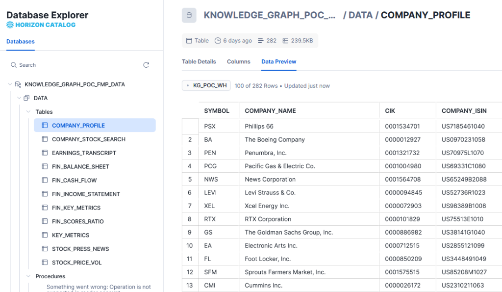
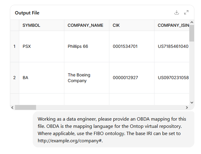
Our space is limited, so we assume you already know how to import data into Snowflake. Here’s a sample of the imported data.

In order to access this data in GraphDB, we would need an interoperability layer. This can be done over the Jata Database Connectivity (JDBC) API. Snowflake offers a JDBC driver. Any recent version would work, but for our tutorial, we’ll use 3.19.1. So, download the driver and place it in the GraphDB distribution directory, under lib/jdbc. No restart is required, GraphDB will dynamically look up JDBC drivers stored there.

Hint: If running on Docker, you can mount the file.
  volumes:

      – ./jdbc:/opt/graphdb/dist/lib/jdbc

 To make the JDBC connection, you need:

• The snowflake URL, which is composed of:
  • The account ID.
  • A static snowflakecomputing.com string.
• The Warehouse identifier.
• The username.
• The password.

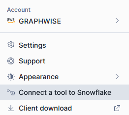
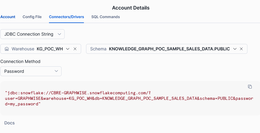
You can get this information (except credentials) from the connectors menu on the bottom left in the Snowflake UI.

Navigate to the Connectors/Drivers tab and select the JDBC Connection String from the dropdown.

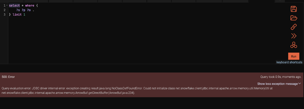
Once you have this information, you can switch to GraphDB. We recommend starting the server with the environment variable JDK_JAVA_OPTIONS=’–add-opens=java.base/java.nio=ALL-UNNAMED’. This is because there is a bug in Snowflake drivers working under Java 16 or later and GraphDB operates on Java 21. If you don’t, you will get an error message when you try to query your virtual repository.

Once you have GraphDB up and running, start by selecting the Setup -> Repositories page from the navigation menu. Create a new Virtual GraphDB repository. Your settings should look similar to this:

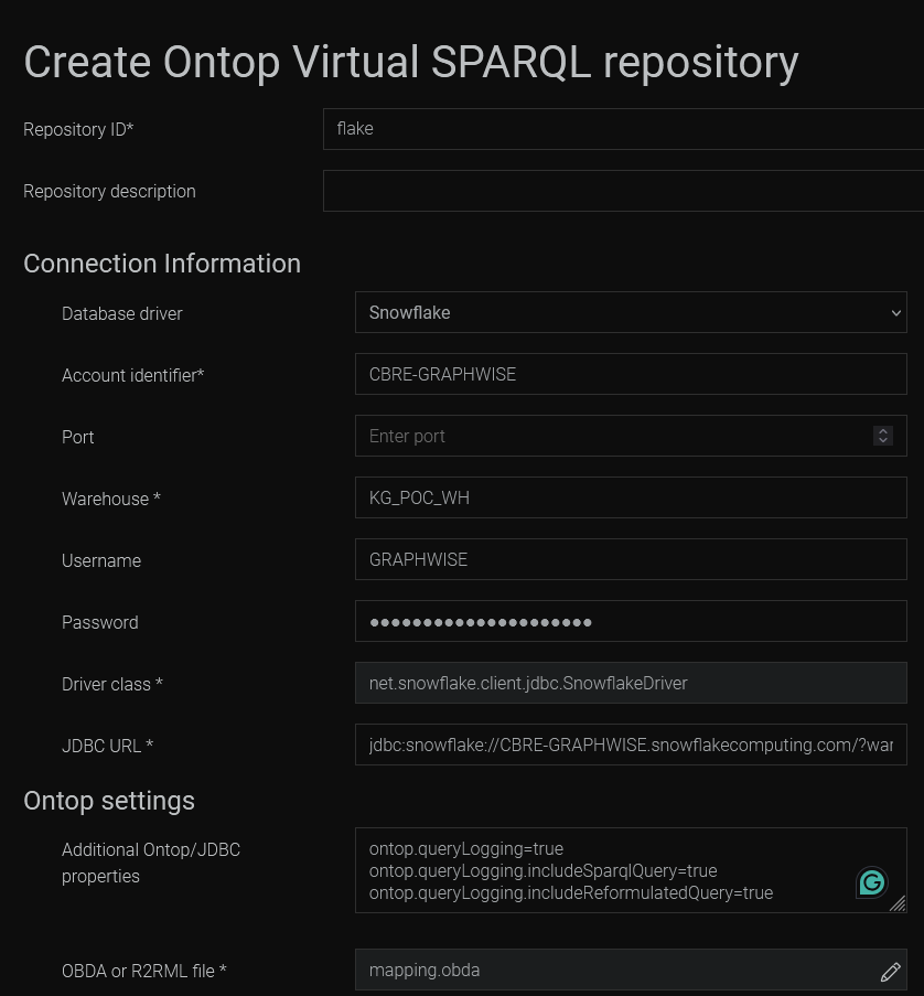
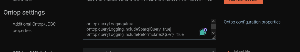
Note the Ontop settings for logging extra information. By default, we have no information about the reformulated query. Configuring those flags would log the queries sent to Snowflake. This is very useful for debugging and the logs only appear when a query is made, so they won’t clutter the general GraphDB log.

Next, we need to write the mapping. We will be using OBDA, the ontop-native mapping language. Ontop is the library embedded in GraphDB to enable integrations of relational data over JDBC.

While this is just a small toy example, following industry standards is a good practice. One of the most important ontologies in the financial domain is FIBO. Using it, we can ensure our data is interoperable with other datasources from the same domain.Writing mapping by hand can be time-consuming and error-prone. For this, we have partnered with Ontopic and we offer the Ontopic studio, which provides syntax assistance and a live preview of the results of your mapping. However, if you want to go even faster, you could start with an LLM prompt.

Be mindful that the initial output likely wouldn’t work out of the box and you would have to refine it in several consecutive iterations. A more efficient approach could be to get the initial mapping from the LLM and carry out alterations by hand.

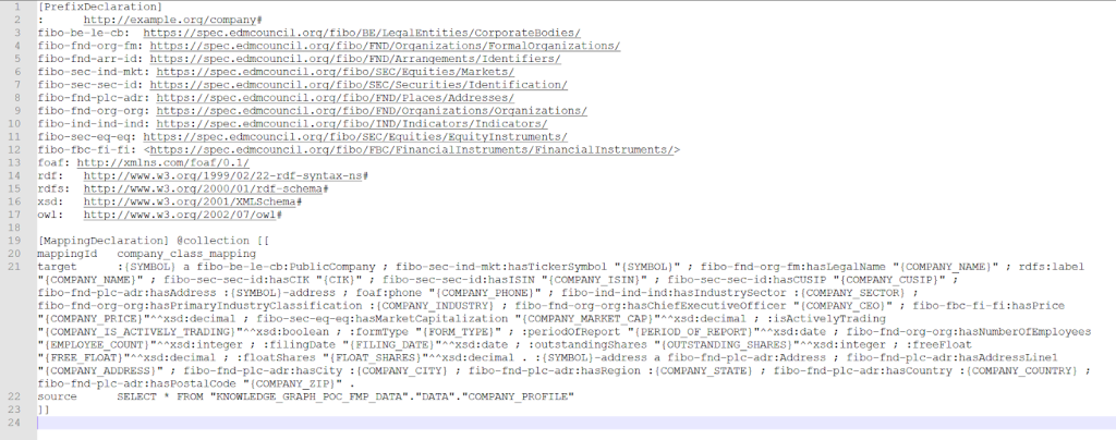
Here’s an example of a mapping.

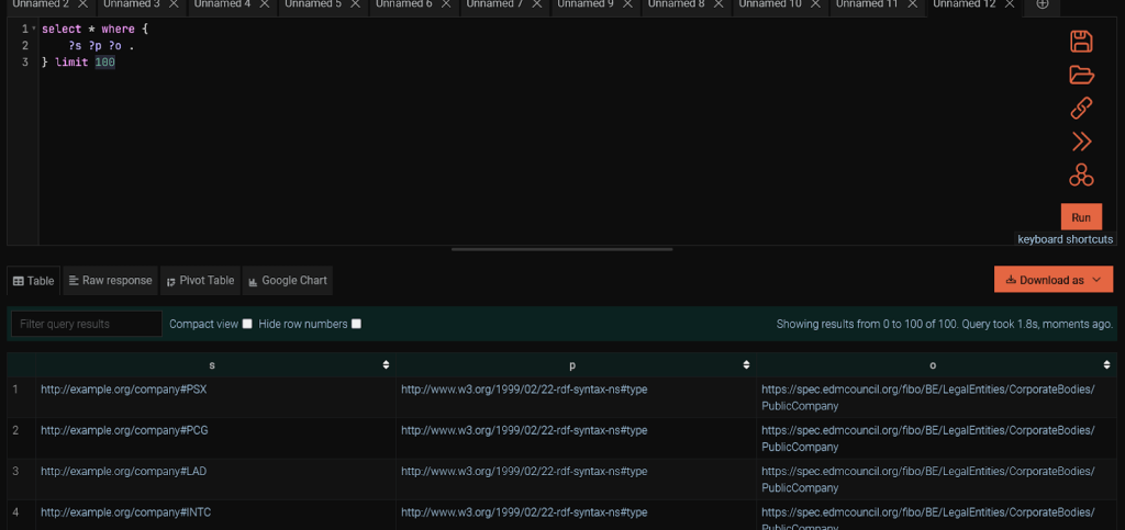
Once you have the mapping and the repository created, let’s fire a simple SPARQL query to ensure it’s properly set up.

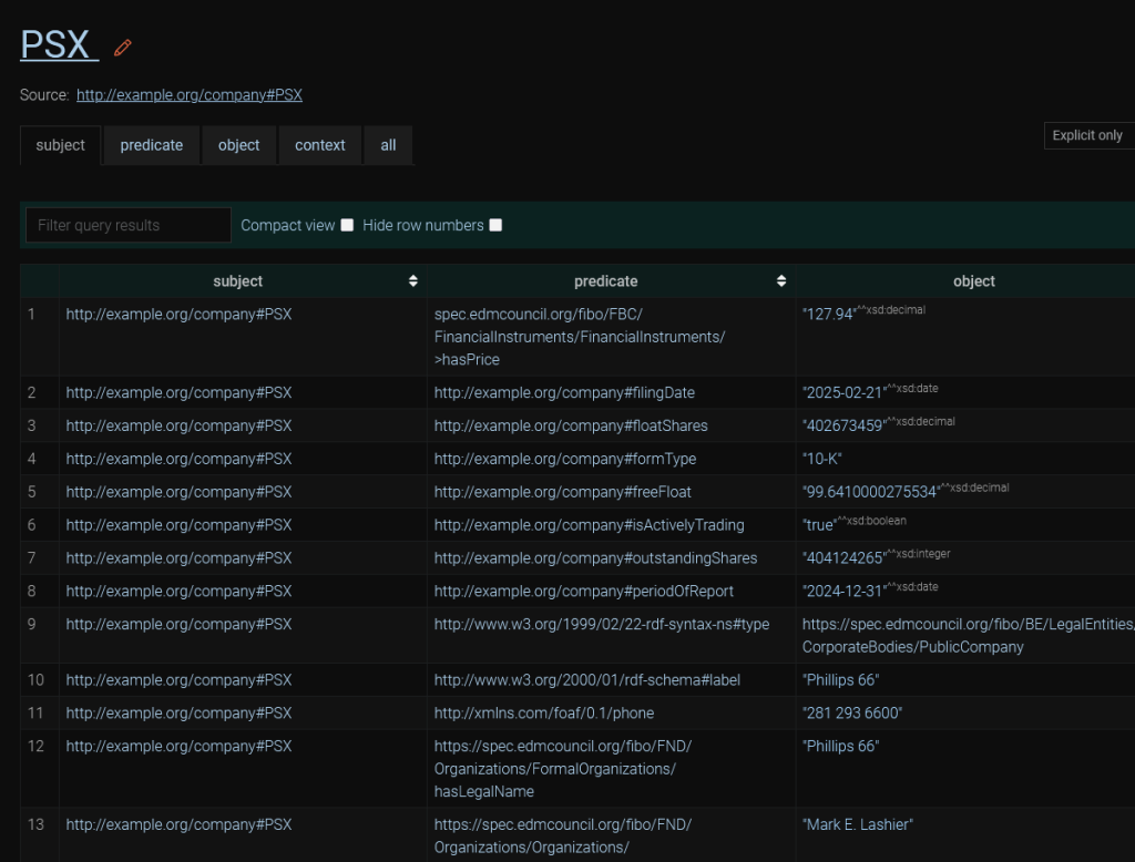
Explore the PSX ticker for extra information.

For the MCP client to write adequate queries, it would need information about the data structure. It could obtain it by running a SPARQL query, which fetches the first 1,000 triples of the database and examining them. However, this is unreliable. There may be predicates (properties) that just aren’t visible in the sample that the LLM picks up. Besides, this would be using up valuable bandwidth and tokens. The best option would be to provide it with an ontology. The GraphDB MCP server exposes a tool that provides ontological data to the LLM. It is based on storing your ontology in a named graph.

We could import the whole FIBO (and friend-of-a-friend) ontologies in graphs and rely on this. However, FIBO and FoaF are large ontologies, and we are using only a small subset of either. Not only would we be wasting tokens on processing the whole ontology, but the LLM may end up writing worse queries since it has parts of the ontology that don’t correspond to any data. 

The best approach would be to take only the parts of FIBO and FoaF that are relevant to our data. We can easily do this with SPARQL, looking up the classes and properties in your triplestore, then deleting all instances from the ontology that are not represented in the data. However, assuming no SPARQL know-how, we could also ask an LLM to do it for you.

Unlike the OBDA mapping, there are a lot of examples of FIBO ontologies available on the Internet and the LLM is much better at writing a correct ontology. It would likely be correct on the first try.

Store this ontology. We would need it shortly.

Relational data materialisation with Refine

Next, we shall store some of our data using an ETL transformation with Refine and import it into a standard GraphDB repository. This serves two purposes.

• It demonstrates another way of integrating data with GraphDB.
• It gives us a repository we can query over MCP.

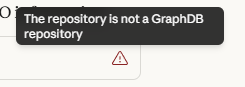
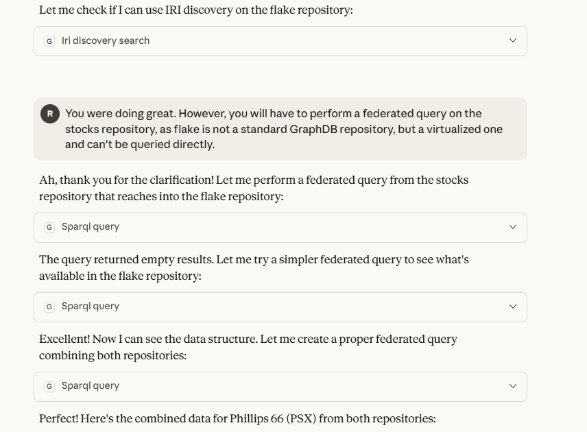
Why the latter purpose? Currently, the MCP server can only work with standard repositories. If it tries to send a query directly to the JDBC-driven virtual repository, we would be presented with an error.

All SPARQL queries would have to use federation and be run on a standard GraphDB repository. Additionally, we can’t import ontologies into the virtual repository. Remember, it is virtual. This means that data is remote and immutable.

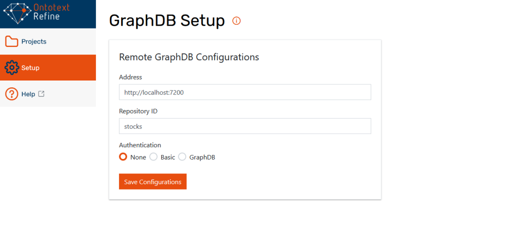
Now that we have explained  the reasons behind creating another repository, let’s go ahead and set it up. First, let’s pick up our CSV. If it is available as a source file, that’s great. Otherwise, we can pick it up from Snowflake using SnowSQL. Once we have the file, start up Refine and configure it to work with GraphDB from the Setup menu.

The next step is to import the file through the Projects menu. Just put in the CSV file and click next.

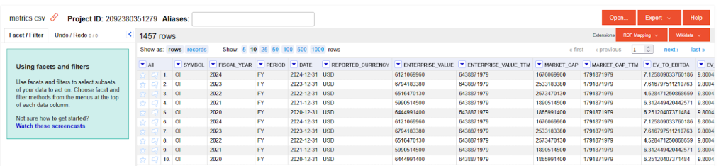
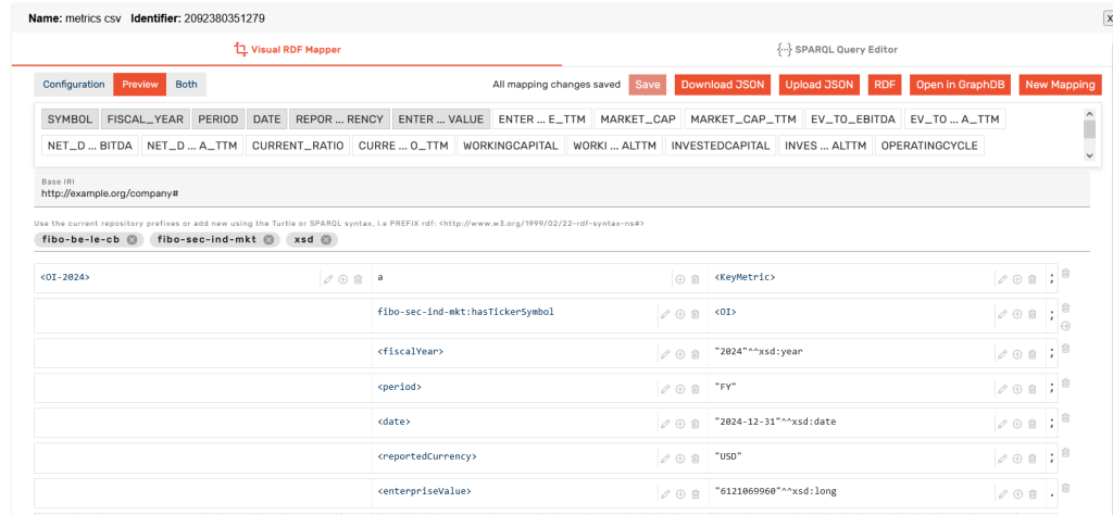
We would not need to perform any modifications on the raw CSV file. Let’s prepare an RDF mapping. Go to the RDF mapper dropdown on the top right. In this graphical mapper, you can drag and drop columns to create RDF from your tabular data. The mapper has a lot of neat features, including a powerful expression language, full operation history, and the capability to export the mapping and reuse it in an ETL pipeline. For more information, you can check out our tutorials on the topic.

Writing the mapping can get tedious when we have hundreds of columns, so it is good to know that you can also automate it with an LLM. The best approach in that case is to use the SPARQL Query editor. First, write a few mappings in the Visual RDF mapper. Switch over to the SPARQL Query Editor and use the Generate Query dropdown to generate a mapping with a service clause.

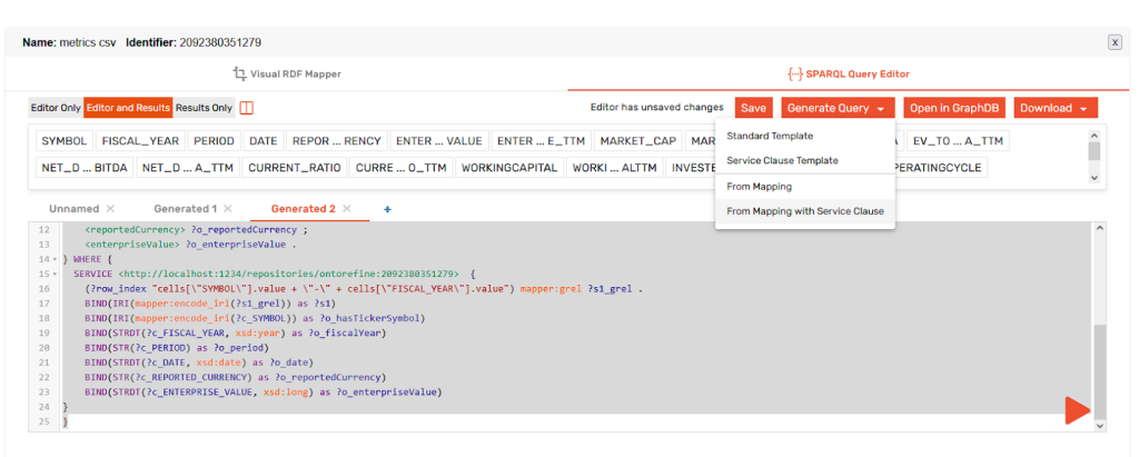
This template, coupled with a sample of the source CSV would be enough for an LLM to write you a SPARQL-based mapping.

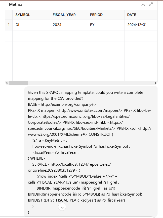
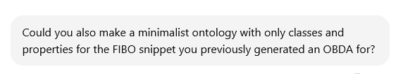
Once you have that, you should ask the LLM for a minimalist ontology as well.

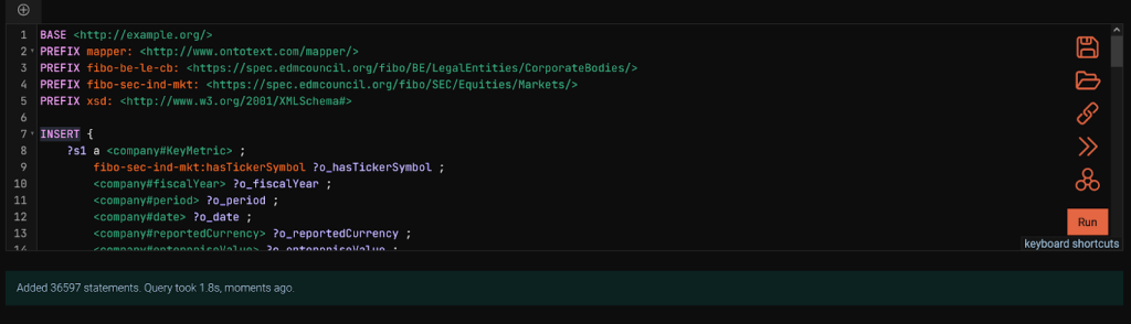
Once we have the mapping ready, we can copy it into GraphDB. We will create a standard repository, calling it stocks. Then, we will go to the SPARQL editor from the navigation menu on the left and paste the mapping. It contains a SPARQL CONSTRUCT. CONSTRUCT is used to display data in RDF format, not to write it to the repository. Let’s run the CONSTRUCT first, to make sure everything looks correct. Then, we will replace the CONSTRUCT keyword with INSERT and materialize the statements.

Remember the two ontologies we created? Now is the time to import them to the repository. Since the virtual repository is not a standard GraphDB repository and thus, can’t be used directly with MCP, we will put its ontology in the new stocks repository.

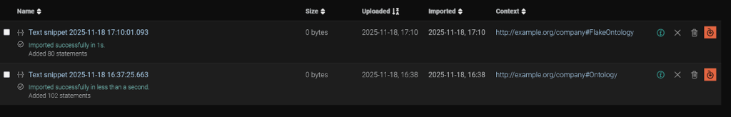
Let’s go to the import menu from the navigation bar, making sure we are on the stocks repository. Then, we can paste the two ontologies – likely in the TTL format – that the LLM provided us with as a text snippet. Remember to import them into two different named graphs. Any name would work, but having a reference to the Flake repository in the name of the ontology graph intended for it would be helpful to the LLM.

Once all that is done, we are finally ready to see the MCP in action.

The MCP client

For this tutorial, we evaluated two MCP clients – LM Studio and Claude. Unfortunately, LM studio is intended for local models. Unless you are running on really powerful hardware, any LLM model you can load into LM studio would not be great at writing SPARQL queries. SPARQL is relatively niche and needs a tailor-made model, or just a very big one. No tailor-made SPARQL-writing LLMs are available and most consumer hardware isn’t powerful enough to host a strong model, so we need a MCP client:

• That can connect to external models.
• And can be run locally.

Why do we care about running locally? Exposing GraphDB to the Internet so a remote MCP client can access it is unnecessary for the purposes of this tutorial and would pad out its length. Suffice it to say, it is as easy as running a GraphDB instance and a gateway service. The MCP server on the GraphDB side has no special configurations necessary. MCP is always-on and applies the security methods available in GraphDB.

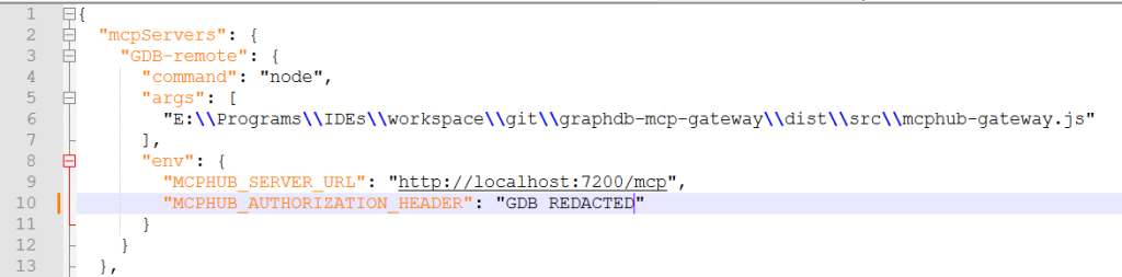
Once we have Claude up and running, we will provide it with the MCP configuration. We can do this by modifying the claude_desktop_config.json.

This file is located under the Claude install directory. On Linux, this is 

~/Library/Application\ Support/Claude

And under Windows, this is

$env:AppData\Claude\

You may notice that we are using the node command with something called the mcphub-gateway. This is because the GraphDB MCP works with the HTTP/SSE protocol, while Claude expects streaming STDIO. The lightweight GraphDB MCP gateway converts requests from one format to the other.

Once we have that configured, the Local MCP server would appear in Claude.

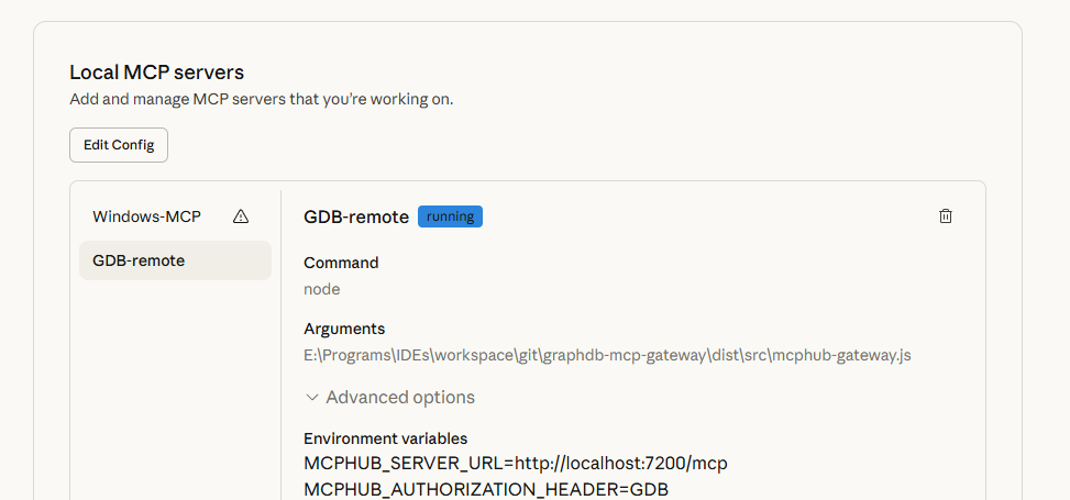
When Claude is set up and the MCP server is running, you can start a new chat. Remember to enable the MCP server connector from the configuration window for this specific chat.

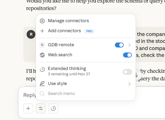
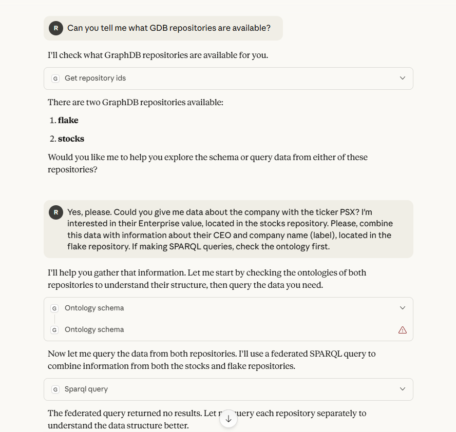
With the MCP server accessible and configured to be used in Claude, you can start making queries.

In case something goes wrong, the Claude logs are available in the Claude installation directory, under logs/main.log and logs/mcp.log.

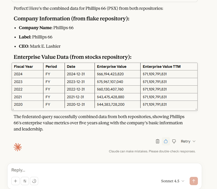
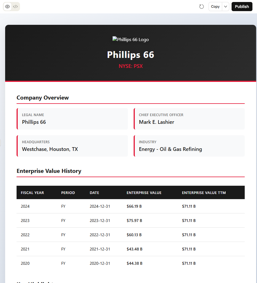
Now that we have unlocked the full power of Retrieval-Augmented Generation (RAG), we can make queries for data available in Snowflake and GraphDB and also combine it with information from the Internet, such as company logos.

Keep in mind that if you are using Claude’s free plan, you will soon hit the session limit.

Wrapping it up

In this tutorial, we have seen how to connect to data in Snowflake with a virtual JDBC repository, how to materialize tabular data using Refine and how to expose this data in a unified view using the MCP Server. 

With that knowledge, what comes next is only up to you.

• Get to know GraphDB better by downloading a local edition.
• Or, perhaps, try out our GraphDB Sandbox. It also has the MCP server enabled!
• Already on GraphDB and following along? Great! You can try adding the Snowflake MCP to your MCP client.

Have questions? Comments? We are always here to help. Reach out via email, phone, LinkedIn, X – if it is a graph of some description, we are on it.

Want to try it for yourself?